Multi-symbol legends in Matplotlib, Python (revised)

[update on 24 May 2025: I realized that some of my old blog posts have been broken due to formatting issues. Hence, I adopted it with the contemporary WordPress writing format in this section. ]

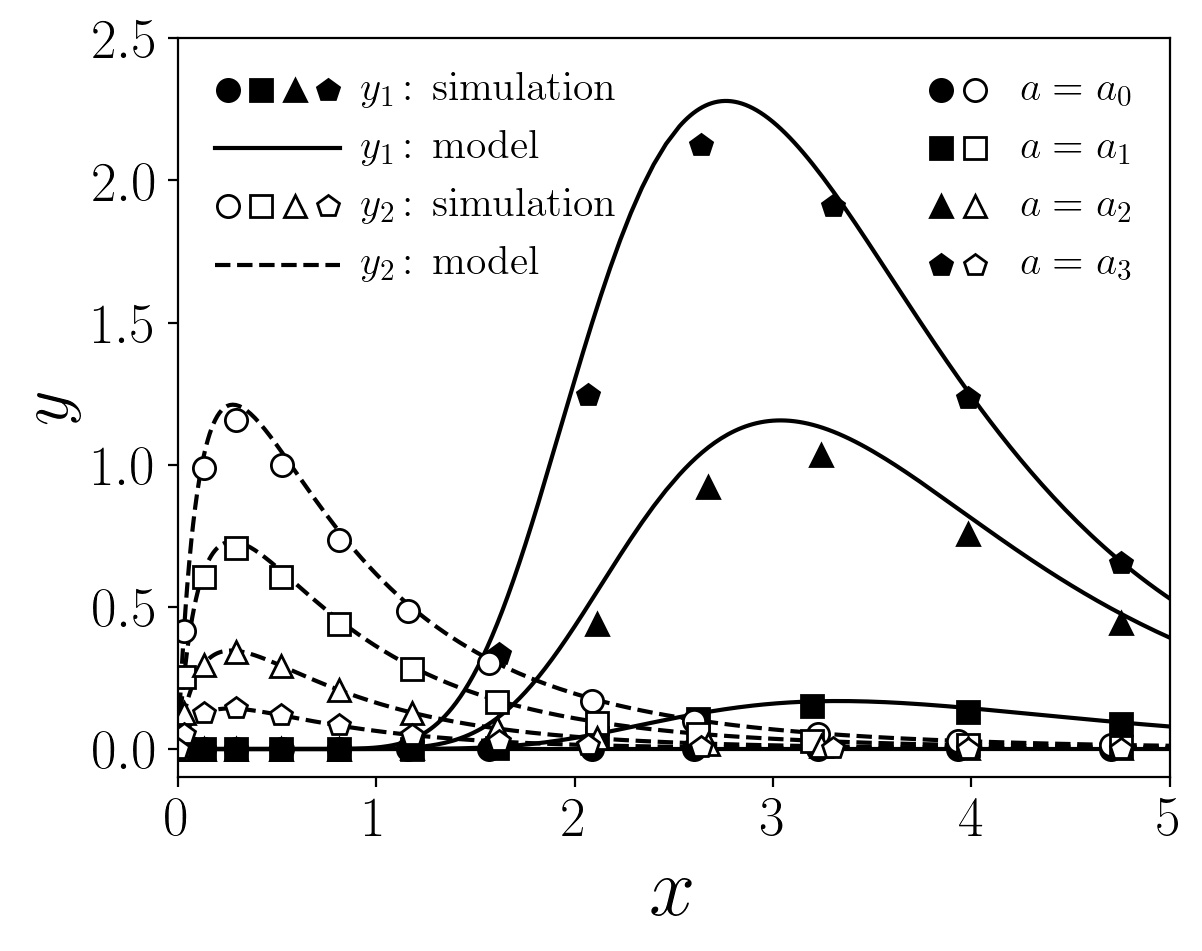
Recently, I met a problem showing multi-dimensional information in a single black-and-white figure. This figure includes (i) simulation data and model predictions for (ii) two different peaks behind the different transport mechanisms (iii) for each given parameter, a=a_0, a_1, a_2, a_3. On top of that, the figure should be black-and-white. Underline these aspects, I found a solution using multi-symbol (or multi-marker) styles in legend, as shown in this figure. Note that the figure below is NOT the one that I am working on. This is an artificial figure for visualization purposes of the contents below.

This black-and-white figure contains multi-dimensional information described above (i-iii). Two peaks y1 and y2 show the opposite trends with respect to ‘a,’ and the agreement between the simulation and model is quite good up to certain order (the original work uses the singular perturbation expansion, so the accuracy there is acceptable with given small parameter). My strategy is to emphasize the two distinct peaks of y1 and y2 by using closed and open symbols for simulation data, and solid and dashed lines for model prediction. Note that symbols make a distinction for different ‘a,’ whereas the lines remain unchanged. Otherwise, the figure became too complicated to deliver a message.

The trick applied to my Python script with matplotlib package is based on this link in Stackoverflow. Using the cleaner solution suggested by tacaswell, the class HandlerXoffset does what I need. Here is my example of using HandlerXoffset originated by tacaswell. The handler p_jq1, p_jq2, … are given by plot itself where I usually use the following:

cnt=0
p_jq1,= plt.plot(x1, y1, symP[cnt], color=colP[cnt], markersize=symsize,
                 markerfacecolor='white', markeredgecolor=colP[cnt]); cnt+=1
p_jq2,= plt.plot(x2, y2, symP[cnt], color=colP[cnt], markersize=symsize,
                 markerfacecolor='white', markeredgecolor=colP[cnt]); cnt+=1
...

where the counter (cnt) usually allocate pre-defined styles colP and symP. Generally speaking, I am using label for each plot, but in this special case, I put the expression on the label directly into the plt.legend(). The first legend located at the upper right corner shows the different types of markers for each a from a_0 to a_3, which is the same between closed and open symbols. For this reason, legend 1 uses both open and closed symbols with an appropriate distance between them. Note that the proper distance is characterized by off_d1 in below, which gives the offset, and the minus sign is which symbols will be located in the first. 

off_d1 = -6.
off_d1 = -6
leg = plt.legend([(p_jq1, p_jb1), (p_jq2, p_jb2), (p_jq3, p_jb3), (p_jq4, p_jb4)],
                 [r'$a=a_0$', r'$a=a_1$', r'$a=a_2$', r'$a=a_3$'],
                 handler_map={p_jq1:HandlerXoffset(x_offset=-off_d1),
                              p_jq2:HandlerXoffset(x_offset=-off_d1),
                              p_jq3:HandlerXoffset(x_offset=-off_d1),
                              p_jq4:HandlerXoffset(x_offset=-off_d1),
                              p_jb1:HandlerXoffset(x_offset=off_d1),
                              p_jb2:HandlerXoffset(x_offset=off_d1),
                              p_jb3:HandlerXoffset(x_offset=off_d1),
                              p_jb4:HandlerXoffset(x_offset=off_d1)},
                 loc = 'upper right', fontsize=15, frameon=False,
                 handlelength=1, markerscale=1.0, handletextpad=1.0)

We can add the additional legend in matplotlib package by using plt.gca().add_artist() as described in below script. In the second legend located at the upper left corner, I would like to show which one belongs to simulation data or model predictions for both y1 and y2. In this case, the distinction based on a is not important. With Handler, all of the markers listed on the legend for each element as shown in the example figure. Note that “handlelength” controls the length of lines or markers whereas “handletextpad” controls the gap between lines/markers and text.

plt.gca().add_artist(leg)
offset_default = -18. # minus sign to make opposite the order of symbols
leg2 = plt.legend([(p_jq1,p_jq2, p_jq3, p_jq4), p1, (p_jb1,p_jb2, p_jb3, p_jb4), p2],
                  [r'$y_1\,\textrm{: simulation}$',r'$y_1\,\textrm{: model}$',  r'$y_2\,\textrm{: simulation}$',r'$y_2\,\textrm{: model}$'],
                  handler_map={p_jq1:HandlerXoffset(x_offset=-offset_default), p_jq2:HandlerXoffset(x_offset=-offset_default/3.),
                               p_jq3:HandlerXoffset(x_offset=offset_default/3.),
                               p_jq4:HandlerXoffset(x_offset=offset_default),
                               p_jb1:HandlerXoffset(x_offset=-offset_default), p_jb2:HandlerXoffset(x_offset=-offset_default/3.),
                               p_jb3:HandlerXoffset(x_offset=offset_default/3.),
                               p_jb4:HandlerXoffset(x_offset=offset_default)},
                  loc='upper left',fontsize=15, frameon=False, handlelength=3,
                  markerscale=1.0, handletextpad=0.5)