I have been using Matplotlib for a long time to produce figures for scientific papers. As a person who is working on the theory and modeling, generating figures using a scripting language minimizes the effort to spend on analysis and produces results. The great flexibility of using a scripting language is a major benefit, regardless of the target format, input data structure, and varying analysis protocols. In this article, some useful figure formats in Matplotlib will be proposed.
The analysis of results is usually done through the visualization of such a numerical value (after some post-processing). In this aspect, we simply generated multiple results file (where their data structure have a shared format structure), the parsing of the list of the filename – which is easily done by bash script – to the post-processing code. I usually decouple the code to generate a figure from that of the post-processing (when the code is almost ready for a certain cycle of research) because of the re-use of such codes with the basic design of the interface between codes.
Underline these aspects, the code templates for figure generation have been distinguished based on the purpose of the figure. For the final results (the figures for conference or scientific papers), all the texts will be treated by LaTeX (inside Matplotlib) because my scientific writing is based on it. The format of sans-serif is described below, where the original description was found in this article.
from matplotlib import rc

rc('font',**{'family':'sans-serif','sans-serif':['Arial']})
rc('text', usetex=True)
plt.rcParams['text.latex.preamble'] = r'''
'''
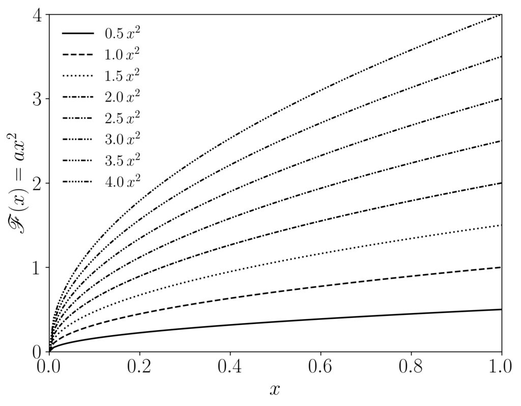
I am the kind of person who produces the figures in black and white unless a colour is absolutely necessary. Matplotlib is versatile tool providing styles of symbols and lines, and also suggest ways of editing details of those presentations. In some cases, I need to show only minor differences between lines (when the conditions are systematically changed), whereas the number of lines is quite large. I found some nice settings on the official Matplotlib site (for details, follow this link).
linestyle_dic = {'-..':(0, (3, 1, 1, 1, 1, 1)),
                 '-...':(0, (3, 1, 1, 1, 1, 1, 1, 1))}

linestyle_dots_dic = {'-.1':(0, (3, 1, 1, 1)),
                      '-.2':(0, (3, 1, 1, 1, 1, 1)),
                      '-.3':(0, (3, 1, 1, 1, 1, 1, 1, 1)),
                      '-.4':(0, (3, 1, 1, 1, 1, 1, 1, 1, 1, 1)),
                      '-.5':(0, (3, 1, 1, 1, 1, 1, 1, 1, 1, 1, 1, 1))}


linestyle_var_dic = {'solid': '-',
                     'loosely dotted':        (0, (1, 10)),
                     'dotted':                (0, (1, 1)),
                     'densely dotted':        (0, (1, 1)),
                     'loosely dashed':        (0, (5, 10)),
                     'dashed':                (0, (5, 5)),
                     'densely dashed':        (0, (5, 1)),
                     'loosely dashdotted':    (0, (3, 10, 1, 10)),
                     'dashdotted':            (0, (3, 5, 1, 5)),
                     'densely dashdotted':    (0, (3, 1, 1, 1)),
                     'dashdotdotted':         (0, (3, 5, 1, 5, 1, 5)),
                     'loosely dashdotdotted': (0, (3, 10, 1, 10, 1, 10)),
                     'densely dashdotdotted': (0, (3, 1, 1, 1, 1, 1))
}
In general, the above settings are saved in an independent file, which is named “plot_default_style.py” in the example below. By doing so, I could keep the same style of the figure for the figures in the same article. This is a general workflow of mine, where independent Python scripts are built for each figure, which share the data and style, but minor post-processing is embedded in the script. Note that the major post-processing is usually done before producing a figure, and results are stored in a shared data. The style usually includes the font size of the label, legend, and tick labels, underlined with the same font size setup. To be specific, one example with different line styles can be found below. Although this sample figure is not suitable for real use, it provides an idea of how to produce different types of lines within the Matplotlib environment. For details, see the code below the figure.

from numpy import *
import matplotlib.pyplot as plt
execfile('plot_default_style_rev.py')

fontsize_label = 20
fontsize_ticks = 20
fontsize_legend = 15

def f(x, a):
    return a*sqrt(x)

plt.close()
# aspect ratio of figsize is 8/6 for most of figures
plt.figure(figsize=(8,6))
plt.ion()

x = linspace(0, 1, 100)

N_con = 8
linP = ['-', '--', ':', linestyle_dots_dic['-.1'], linestyle_dots_dic['-.2'], \
        linestyle_dots_dic['-.3'], linestyle_dots_dic['-.4'],                 \
        linestyle_dots_dic['-.5']]

# # when various types are necessary
# linP = [linestyle_tuple['solid'], linestyle_tuple['densely dashed'],                 \
#         linestyle_tuple['densely dotted'], linestyle_tuple['densly dashdotted'],     \
#         linestyle_tuple['densely dashdotdotted'], linestyle_tuple['densely dotted'], \
#         linestyle_tuple['densely dashed'], linestyle_tuple['densely dotted']]

a_arr = linspace(0.5, 4.0, N_con)


for i in range(N_con):
    plt.plot(x, f(x, a_arr[i]), 'k', linestyle=linP[i], label = r'$

# arguments: location of legned, fontsize, line for frame, number of columns
plt.legend(loc = 'upper left', fontsize=fontsize_legend, frameon=False, ncol=1)


plt.xlabel(r'$x$', fontsize=fontsize_label)
plt.ylabel(r'$\mathscr{F}(x) = ax^2$', fontsize=fontsize_label)

plt.yticks(arange(0, 4.1, 1))
plt.tick_params(labelsize=fontsize_ticks)
plt.axis([0, 1, 0, 4])
plt.savefig('tmp.jpg', bbox_inches='tight', dpi=300)
# plt.savefig('tmp.tiff', bbox_inches='tight', dpi=300)
# plt.savefig('tmp.pdf', bbox_inches='tight')
# # for eps setting
# plt.savefig('tmp.eps', format='eps', dpi=300)
plt.show()
In summary, the font setting with the LaTeX setting has been addressed. The default format and workflow for figure processing are (minorly) described. The detailed description of linestyle is added with a working example of the code. In the future, the detailed workflow and general idea to produce a clear figure will be addressed.

Leave a Reply